Data structures & Algorithms (DSA) may be the bain of every computer science student's existence; it sure was mine. But after contributing to/writing software for small businesses and personal projects, I can appreciate why it's important to learn and its specific use cases. DSAs allow us to have a structured approach when trying to solve a problem. Whether you are trying to solve the next Leetcode problem or help a business design new software, understanding DSAs serves an important role in software engineering. This article will explore the sorting algorithms part of DSA's and tour through the importance and use cases of various sorting algorithms.

So that we are on the same page, let's first define an algorithm: it is a set of instructions that define how a task is to be completed. We're met with algorithms in our daily lives without even thinking about it. For example, think about a chore that is part of your weekly routine -- if you were to automate this chore, how would you go about doing it? What's the first thing you would do? What are the steps in the middle? What's the final step? The list of instructions that you come up with is essentially an algorithm -- a set of instructions that define how to complete a task.

Focusing more on computer science topics, there are many different algorithms that allow us to complete various tasks. One common task for computer scientists/programmers is sorting an iterable list using one of the various sorting algorithms. There are quite a few sorting algorithms and so the question becomes does it really matter which one we pick to solve our problem? I mean at the end of the day we're still sorting a list. In short, yes it matters which sorting algorithm is picked to solve the problem but I think it's more nuanced as it all stems back to the point of efficiency. Although there are many sorting algorithms to choose from, some algorithms are more efficient than others. But how do we determine how efficient an algorithm is?

Big O notation

The efficiency of an algorithm is measured in a notation known as Big O and it's really meant to describe the behaviour of a function/algorithm as the input size grows to infinity. It's used both in computer science and mathematics and it becomes very useful when thinking about how to design scalable algorithms/functions. The algorithm you design might work well when the input size is small but how does it perform as the input size grows? That's what big O aims to answer and it's why we look at an input size of infinity when assessing efficiency.

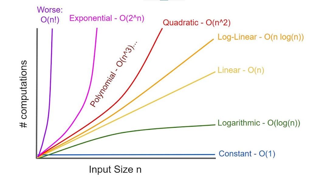
Below is an image describing the different Big O notations where the x-axis represents the number of operations and the y-axis represents the performance of the function/algorithm. When we refer to the different big O notations, you will often see it denoted as O(n) where O represents the order of magnitude and n represents the number of operations in an algorithm.

Let's say we had a phone book and we wanted to search for a particular name, how would we go about doing it?

1. We could be given the exact location of that name in the phonebook. That way we just have to go to that page and retrieve the information

2. We go look through the phonebook page by page to find the name and information that interests us

3. Assuming the phone book is sorted in alphabetical order, we could use a narrowing down method. We could open the phone book to the middle page and check if the name we want is less than or greater than the names in the middle. Depending on the section, we then open the middle of that respective section; narrowing it down until we find the name of interest.

Of the approaches listed above, one of them is clearly more efficient while other approaches require more steps/operations to accomplish the same task. When designing algorithms, it's important to think about how these algorithms are going to scale and how performant they are going to be at large input sizes. For a phonebook that does not have many pages, option 2 may be a viable method but that becomes less the case as the phonebook grows in size.

Common Big O complexity

We're going to be looking at some of the common Big O complexities and exploring what they mean on an individual level.

O(1)

O(1) also known as constant time describes an algorithm that does not change in performance as the input size grows to infinity. These algorithms are very efficient as an input of size 10 and an input size of 1,000,000 will have the same performance.

An example of an operation that has a constant time complexity is looking up an item in an array where we have the index (the location of the item). Since we have the index of the item we want to search for, the size of the array becomes irrelevant as getting the item we want just requires us to go to the location/index in the array, therefore this operation takes the same amount of time. Using the example described above with the phonebook, we can see that option 1 has a constant time operation.

O(log n)

O(log n) also known as logarithmic time describes an algorithm whose performance grows half as fast in proportion to the size of the input. Therefore, at very large input sizes, the change in performance of a logarithmic algorithm is small. You mostly see logarithmic functions in recursive functions and binary search algorithms. Using the example described above with the phonebook, we can see that option 3 operates in logarithmic time.

In computer science when we speak of logarithms, we assume a base of 2 unless otherwise stated.

O(n)

O(n) also known as linear time describes an algorithm whose performance grows linearly and in direct correlation to the input size. Therefore, the increased input size leads to a proportional increase in run time. Going back to the scenario above, looking through the phonebook page by page to find your name of interest would have a time complexity of O(n). Since it would take n operations to find the name of interest in a phone book of size n names. A common example of an O(n) operation is iterating a list of size n to do some operation. Using the example described above with the phonebook, we can see that option 2 operates in linear time.

O(n log n)

O(n log n) also known as log-linear time describes an algorithm that performs log n operations n times. The run time of an algorithm with this time complexity grows with the size of the input (almost linearly) although we perform a log n operation at each step. We are performing extra steps when compared to an O(n) time complexity therefore we say that an algorithm with an O(n log n) time complexity is less efficient than an algorithm with an O(n) time complexity.

O(n^2)

O(n^2) also known as quadratic time describes an algorithm whose performance exponentially increases in correlation with the input size. The performance of the algorithms gets much slower as the input size grows to infinity. At every step, we perform an n operation therefore we say that an algorithm with an O(n^2) time complexity is less efficient than an algorithm with an O(n) or O(n log n) time complexity. This is commonly seen with nested loops although nested loops do not always mean a time complexity of O(n^2).

Sorting Algorithms

As I alluded to above, a common thing that computer programmers do is retrieve data, sort data, and search through data. Many sorting algorithms can be used to complete these tasks and it's left to the developer to decide & implement the appropriate one for the job. To appropriately make this decision, the developer must think about how the data will scale because this choice will impact the efficiency of the overall application.

Below are some examples of sorting algorithms that are available for use. This is just a very short list so there are more than just the ones listed below.

Bubble Sort

I find that bubble sort is the easiest sorting algorithm to conceptually think about as larger items are progressively being moved to the top of the list. People often say that with bubble sort larger items are bubbled up to the top. Bubble sort compares two adjacent elements and if the current item in the list is greater than the next item in the list, a swap will occur. This is done for the entire length of the list, thus leading to a sorted list.

Suppose we are trying to sort the following array of numbers in ascending order, using bubble sort the following will occur:

1. Starting from the first index, compare the first and the second elements.
2. If the first element is greater than the second element, they are swapped.
3. Now, compare the second and the third elements. Swap them if they are not in order.
4. The above process goes on until the last element.

Using the demo below, try to implement the bubble sort algorithm.

This occurs for the length of the entire list and until the entire list is sorted. In its worst case, the bubble sort algorithm has a time complexity of O (n^2), therefore it would not be recommended for use with large data sets. As mentioned above an algorithm with a time complexity of O(n^2) does not scale very well.

Selection Sort

Selection sort selects the smallest element from an unsorted list in each iteration and places that element at the beginning of the unsorted list.

Suppose we are trying to sort the following array of numbers in ascending order, using selection sort the following will occur:

1. Set the first element in the list as the minimum value
2. Compare minimum with the second element. If the second element is smaller than minimum, assign the second element as minimum.
3. Compare minimum with the third element. Again, if the third element is smaller, then assign minimum to the third element otherwise do nothing. The process continues until the last element.
4. The minimum item is moved/swapped into the sorted half of the list -- this is in front of the first unsorted item in the list.
5. Indexing then starts from the first unsorted item and steps 1 - 4 are repeated.
6. This occurs for the length of the entire list and until the entire list is sorted.

Below you will find an interactive example of selection sort in action. The green inner box represents the sorted array that is going to be created while the outer box represents the unsorted array. Drag the following numbers into the sorted array section and at each iteration, you're going to pick the smallest number from the unsorted array section.

In its worst-case and best-case, the selection sort algorithm has a time complexity of O (n^2). The time complexity of the selection sort is the same in all cases as at every step, you have to find the minimum element and put it in the right place. The minimum element is not known until the end of the array is not reached. Therefore, this algorithm would not be recommended for use with large data sets.

Insertion sort

Insertion sort places an unsorted element at its suitable place in each iteration -- it works similarly as we sort cards in our hand in a card game.

Suppose we are trying to sort the following array of numbers in ascending order. Using insertion sort the following will occur:

1. We split our unsorted list into a sorted and unsorted section
2. We assume that the first item in the list is already sorted so we look at the second item
3. We move the second item( herein denoted as currItem) into the sorted section of the list and compare it to previous values in the sorted section
4. If the currItem is less than its previous value, then we swap the previous value with currItem
5. This is done for the entire length of the sorted section. If currItem is greater than its previous value then we stop and move on to the next item in the unsorted section

This occurs for the length of the entire list and until the entire list is sorted. In the demo below, you can drag the numbers around to get a sense of how to implement the insersion sort algorithm.

In its worst case, the insertion sort algorithm has a time complexity of O (n^2) while in its best case the insertion sort algorithm has a time complexity of O(n). The worst-case may occur if you want to reserve an array that is in ascending order -- put the array into descending order. Each element has to be compared with the other elements thus leaving you with n(n-1) -- this gives you the n^2 time complexity. The best case may occur if the array is already sorted since you would not need to perform a sort in the sorted section of the array.

Quick Sort

The quick sort algorithm is based on the Divide and Conquer paradigm as the array is initially divided into two halves and then later combined in a sorted manner. It selects an element as a pivot value and then partitions the given array around the selected pivot value. Elements that are less than the pivot are placed to the left while elements that are greater than the pivot are placed to the right of the pivot element. This way the pivot value is considered sorted.

Here's a guide to the first iteration of the quick-sort algorithm. From the number is the array presented below,

1. select a pivot value
2. move all the elements that are less than the pivot to the left box
3. move all the elements that are greater than the pivot value to the right box
4. This is done recursively until the entire array/list has become sorted.

In its worst case, the quick sort algorithm has a time complexity of O (n^2) since there may be a case where the pivot element selected is the greatest or smallest element in the list. This creates a case where all the elements are on the extreme end of the array thus having one sub-array always being empty while the other contains n-1 elements. For this reason, the quicksort algorithm is best performed when there are scattered pivot points. In its best case, the quick sort algorithm has a time complexity of O(n log n) since there may be cases where the pivot element selected is always the middle element or near to the middle element.

On average quicksort has a time complexity of O(n log n) and a space complexity of O(log n).

Merge Sort

The merge sort algorithm is based on the Divide and Conquer paradigm as the array is initially divided into two halves and then later combined in a sorted manner. It's often thought of as a recursive algorithm that constantly splits an array or sub-arrays into smaller units until it reaches the base case where it cannot be divided anymore. The individual items are then merged back together in sorted order which produces the original array that is now sorted. Below is an image describing the merge sort algorithm.

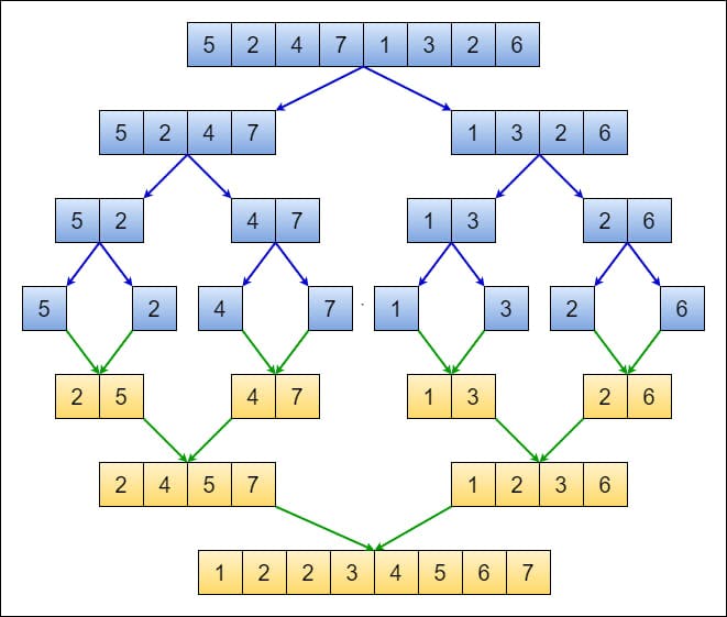
In its worst-case and best-case, the merge sort algorithm has a time complexity of O(n log n). This is really good in terms of efficiency, however, merge sort also has a space complexity of O(n). Therefore, as the input size grows, the space needed to complete this algorithm grows proportionally. Essentially we're making a tradeoff in terms of efficiency for space.

To wrap up

Algorithms are very useful functions that abstract away a lot of logic and they make developer lives so much easier. Algorithms allow developers to write instructions once and then implement them everywhere thereby allowing developers to focus on writing the application. The best algorithm takes into account how the data it receives will scale so as to maximize efficiency. So, whether you are trying to solve the next Leetcode problem or help a business design new software, understanding how to best implement algorithms serves an important role in software engineering.

Hope you found this useful, don't forget to smash the like button and I'll catch you in the next one... Peace!